Various Models of Linear Logic
Classical/Intuitionistic logic is governed by a set of structural and logical rules. The logical rules comprise modus ponens, $\wedge$, $\vee$, and $\bot$. The structural rules comprise contraction, weakening, and exchange. The rules for each are as follows, respectively:
$$ \frac{\Gamma, A, A \vdash \Delta}{\Gamma, A \vdash \Delta}, \qquad \frac{\Gamma \vdash \Delta}{\Gamma, A \vdash \Delta}, \qquad \frac{\Gamma, A, B, \Sigma \vdash \Delta}{\Gamma, B, A, \Sigma \vdash \Delta}. $$
Linear logic, however, refines classical/intuitionistic logic by omitting the contraction and weakening rules. Thus, linear logic strictly requires every premise to be used exactly once.
A natural question to ask is why use a more restricted logic? Yves Saint Girard motivates linear logic via resource availability. $A \vdash B$ can be interpreted as using resource $A$ to make available resource $B$. During this process, it is possible that resource $A$ changes or gets consumed. Ergo, linear logic allows us to refrain from duplicating or discarding resources.
Propositions for Linear Logic
The propositions for linear logic are as follows:
| Symbol | Read as | Name |
|---|---|---|
| Every propositional variable is a proposition. | ||
| $A^{\perp}$ | negation | Negation of $A$ |
| For propositions $A$ and $B$: | ||
| $A \& B$ | with | Additive conjunction of $A$ and $B$ |
| $A \oplus B$ | plus | Additive disjunction of $A$ and $B$ |
| $A \otimes B$ | times | Multiplicative conjunction of $A$ and $B$ |
| $A ⅋ B$ | par | Multiplicative disjunction of $A$ and $B$ (also $A \mid B$) |
| Constants: | ||
| $\top$ | top | Additive truth |
| $0$ | zero | Additive falsity |
| $1$ | one | Multiplicative truth |
| $\bot$ | bottom | Multiplicative falsity |
| For each proposition $A$: | ||
| $!A$ | of course | Exponential conjunction of $A$ |
| $?A$ | why not | Exponential disjunction of $A$ |
It is reasonable to think this is too restrictive a framework. Linear logic addresses this through its exponential modalities, particularly the operator $!A$, read as of course. The exponential makes it possible to recover behavior that is normally excluded. Thus, we don't completely abandon contraction and weakening, but we control when they can be employed.
Another important property of linear logic is linear negation. The negation of a proposition $A$ is written $A^\perp$. Linear negation can be understood operationally in terms of inputs and outputs. One way of viewing it is as swapping their roles, where what was regarded as an input is now regarded as an output, and vice versa. This helps us interpret propositions as interfaces between processes instead of some static truth value.
One of the advantages of linear logic is its relationship with parallelism. Linear transformations can be reversed as resources cannot simply disappear or be duplicated. Thus, we can consider transformations in both directions, which is nonstandard in ordinary typed lambda calculus. Consider the following example: suppose we have a term whose type can be viewed as a transformation from a "question" to an "answer." This transformation needn't be linear, but linear logic allows you to reverse the roles of "question" and "answer."
The following discussion concerns the various models of linear logic.
Model 1: Linear Algebra
The category of finite-dimensional vector spaces over finite fields is a model of linear logic. This makes sense at a high level since vector spaces come equipped with operations that behave like the tensorial and additive structure appearing in linear logic, while linear maps provide a natural interpretation of transformations between resources. The objects of the relevant monoidal category are finite-dimensional vector spaces over finite fields, and the morphisms are linear maps.
A vector space can also be described using coordinates indexed by a set $X$. Choosing an appropriate basis gives a concrete way to represent the space and its linear maps. We initially frame it in a category-theoretic fashion to see how the structural rules of linear logic appear in linear algebra.
The Exponential $!A$ and Finite Multisets
Recall that linear logic normally does not allow us to duplicate a resource, but $!A$ allows us to wisely use weakening and contraction. It follows that the coordinate set associated with $!A$ should therefore consist of finite multisets of elements drawn from $A$. This is true because $!A \cong 1 \& A \& A^2 \& A^3 \& \cdots$ as $!A$ allows us to have zero, one, two, three, or arbitrarily many copies of $A$. Consequently, the set $⟦ !A \rrbracket$ can be viewed as the set of finite multisets whose elements come from $⟦ A \rrbracket$. A multiset makes sense here because the number of copies of an element matters ( for resource consumption purposes, ${a,a}$ is different from ${a}$). Thus, the coordinate set of the vector space corresponding to $!A$ should, morally, consist of finite multisets drawn from $A$. Each basis element can therefore be thought of as representing a particular finite collection of resources from $A$. The empty multiset corresponds to weakening, while multisets containing multiple copies correspond to contraction. Finally, if $A$ is interpreted as a vector space with dimension $\dim ⟦ A \rrbracket$, then the corresponding vector space over the finite field $\mathbb{F}_q$ has $ q^{\dim ⟦ A \rrbracket} $ elements.
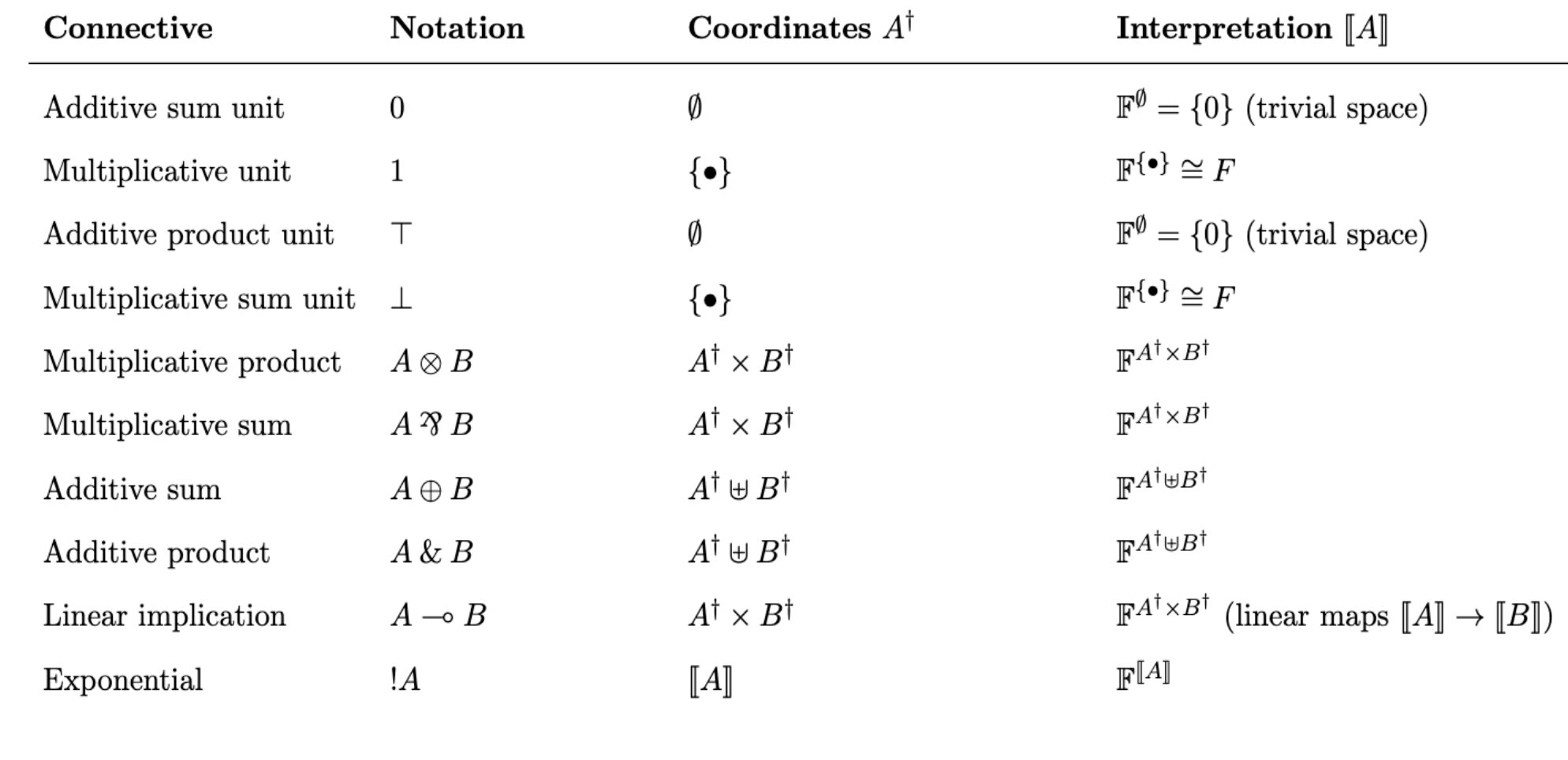
For weakening and contraction, note that $$ \frac{\Gamma \otimes 1 \vdash B} {\Gamma \otimes !A \vdash B} $$ is equivalent to $$ \varepsilon : !A \to 1. $$ and $$ \frac{\Gamma \otimes (!A \otimes !A) \vdash B} {\Gamma \otimes !A \vdash B} $$ is equivalent to the diagonal map $$ \delta_v \mapsto \delta_v \otimes \delta_v. $$ respectively. Other connections from linear algebra to linear logic are shown in the image below, comparing linear logic and linear algebra.
Model 2: Geometry of Interaction
The finite-dimensional vector-space construction can be viewed as a denotational or categorical model where propositions and proofs are interpreted as mathematical objects and morphisms. Geometry of Interaction (GoI), by contrast, is presented as a dynamical model. In this perspective, instead of considering a proof of a linear entailment $A \vdash B$ as a morphism between objects $A$ and $B$ in a monoidal category as in categorical semantics, a proof can be regarded as an endomorphism on an object $A \multimap B$ (operational semantics).
Consider $\mathcal{C}$ to be a traced monoidal category. Then, $\operatorname{Int}(\mathcal{C})$ denotes the compact, closed category generated by $\mathcal{C}$, where the objects are of the form $(A^+, A^-)$, and the morphisms are of the form
$$ (A^+ \otimes B^-) \longrightarrow (A^- \otimes B^+). $$
The subcategories are useful in formalizing linear maps on spaces of operators on Hilbert spaces that take density matrices to density matrices. The subcategories are famous in quantum physics as categories of superoperators or categories of quantum operations. Thus, it has relations to quantum physics.